Math Node
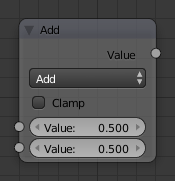
Math node.
This node performs math operations.
Inputs
- Value
- First numerical value. The trigonometric functions accept values in radians.
- Value
- Second numerical value. This value is not used in functions that accept only one parameter like the trigonometric functions, Round and Absolute.
Properties
- Operation
- Add, Subtract, Multiply, Divide, Sine, Cosine, Tangent, Arcsine, Arccosine, Arctangent, Power, Logarithm, Minimum, Maximum, Round, Less Than, Greater Than, Modulo, Absolute.
- Clamp
- Limits the output to the range (0 to 1). See clamp.
Outputs
- Value
- Numerical value output.
Examples
Manual Z-Mask
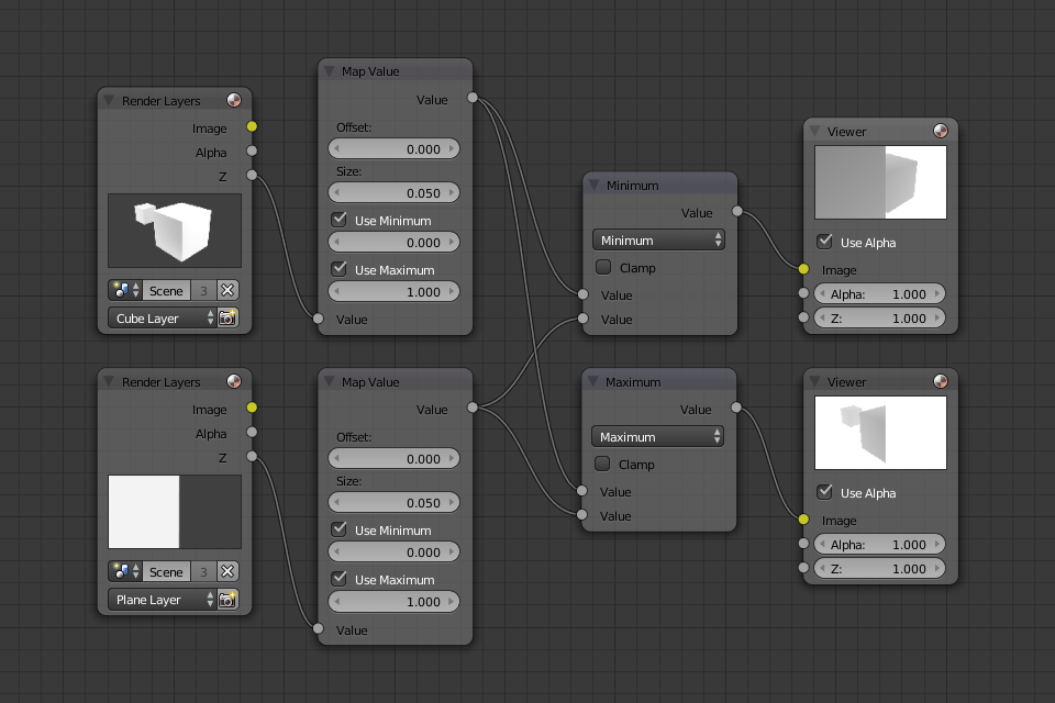
Example.
This example has one scene input by the top Render Layer node, which has a cube that is about 10 BU from the camera. The bottom Render Layer node inputs a scene (FlyCam) with a plane that covers the left half of the view and is 7 BU from the camera. Both are fed through their respective Map Value nodes to divide the Z buffer by 20 (multiply by 0.05, as shown in the Size field) and clamped to be a min/ max of 0.0/ 1.0 respectively.
For the minimum function, the node selects those Z values where the corresponding pixel is closer to the camera; so it chooses the Z values for the plane and part of the cube. The background has an infinite Z value, so it is clamped to 1.0 (shown as white). In the maximum example, the Z values of the cube are greater than the plane, so they are chosen for the left side, but the plane (FlyCam) Render layers Z are infinite (mapped to 1.0) for the right side, so they are chosen.
Using Sine Function to Pulsate
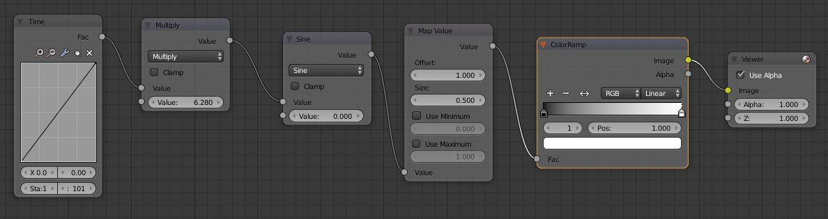
This example has a Time node putting out a linear sequence from 0 to 1 over the course of 101 frames. The green vertical line in the curve widget shows that frame 25 is being put out, or a value of 0.25. That value is multiplied by 2 × pi and converted to 1.0 by the Sine function, since we all know that \(sin(2 × pi/ 4) = sin(pi/ 2) = +1.0\) Since the sine function can put out values between (-1.0 to 1.0), the Map Value node scales that to 0.0 to 1.0 by taking the input (-1 to 1), adding 1 (making 0 to 2), and multiplying the result by one-half (thus scaling the output between 0 to 1). The default Color Ramp converts those values to a grayscale. Thus, medium gray corresponds to a 0.0 output by the sine, black to -1.0, and white to 1.0. As you can see, \(sin(pi/ 2) = 1.0\). Like having your own visual color calculator! Animating this node setup provides a smooth cyclic sequence through the range of grays.
Use this function to vary, for example, the alpha channel of an image to produce a fading in/out effect. Alter the Z channel to move a scene in/out of focus. Alter a color channel value to make a color “pulse”.
Brightening/Scaling a Channel
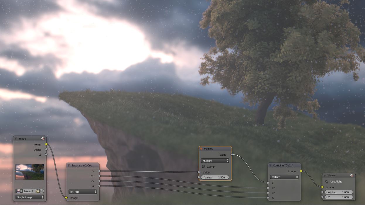
This example has a Math: Multiply node increasing the luminance channel (Y) of the image to make it brighter. Note that you should use a Map Value node with min() and max() enabled to clamp the output to valid values. With this approach, you could use a logarithmic function to make a high-dynamic range image. For this particular example, there is also a Brighten/Contrast node that might give simpler control over brightness.
Quantize/Restrict Color Selection
In this example, we want to restrict the color output to only 256 possible values. Possible use of this is to see what the image will look like on an 8-bit cell phone display. To do this, we want to restrict the R, G and B values of any pixel to be one of a certain value, such that when they are combined, will not result in more than 256 possible values. The number of possible values of an output is the number of channel values multiplied by each other, or Q = R × G × B.
Since there are three channels and 256 values, we have some flexibility how to quantize each channel, since there are a lot of combinations of R × G × B that would equal 256. For example, if {R, G, B} = {4, 4, 16}, then \(4 × 4 × 16 = 256\). Also, {6, 6, 7} would give 252 possible values. The difference in appearance between {4, 4, 16} and {6, 6, 7} is that the first set (4, 4, 16} would have fewer shades of red and green, but lots of shades of blue. The set {6, 6, 7} would have a more even distribution of colors. To get better image quality with fewer color values, give possible values to the predominant colors in the image.
Theory
Two Approaches to Quantizing to six values.
To accomplish this quantization of an image to 256 possible values, let us use the set {6, 6, 7}. To split up a continuous range of values between 0 and 1 (the full Red spectrum) into six values, we need to construct an algorithm or function that takes any input value but only puts out six possible values, as illustrated by the image to the right. We want to include zero as true black, with five other colors in between. The approach shown produces {0, 0.2, 0.4, 0.6, 0.8, 1}. Dividing 1.0 by 5 equals 0.2, which tells how far apart each quantified value is from the other.
So, to get good even shading, we want to take values that are 0.16 or less and map them to 0.0; values between 0.16 and 0.33 get fixed to 0.2; color band values between 0.33 and 0.5 get quantized to 0.4, and so on up to values between 0.83 and 1.0 get mapped to 1.0.
Note
Function f(x)
An algebraic function is made up of primitive mathematical operations (add, subtract, multiply, sine, cosine, etc) that operate on an input value to provide the desired output value.
Spreadsheet showing a function.
The theory behind this function is scaled truncation. Suppose we want a math function that takes in a range of values between 0 and 1, such as 0.552, but only outputs a value of 0.0, 0.2, 0.4, etc. We can imagine then that we need to get that range 0 to 1 powered up to something 0 to 6 so that we can chop off and make it a whole number. So, with six divisions, how can we do that? The answer is we multiply the range by 6. The output of that first math Multiply Node is a range of values between 0 and 6. To get even divisions, because we are using the rounding function (see documentation above), we want any number plus or minus around a whole number will get rounded to that number. So, we subtract a half, which shifts everything over. The round() function then makes that range 0 to 5. We then divide by 5 to get back a range of numbers between 0 and 1 which can then be combined back with the other color channels. Thus, you get the function \(f(x, n) = round(x × n - 0.5)/ (n - 1)\) where “n” is the number of possible output values, and “x” is the input pixel color and \(f(x, n)\) is the output value. There is only one slight problem, and that is for the value exactly equal to 1, the formula result is 1.2, which is an invalid value. This is because the round function is actually a roundup function, and exactly 5.5 is rounded up to 6. So, by subtracting 0.501, we compensate and thus 5. 499 is rounded to 5. At the other end of the spectrum, pure black, or 0, when 0.501 subtracted, rounds up to 0 since the Round() function does not return a negative number.
Sometimes using a spreadsheet can help you figure out how to put these nodes together to get the result that you want. Stepping you through the formula for \(n = 6\) and \(x = 0.70\), locate the line on the spreadsheet that has the 8-bit value 179 and R value 0.7. Multiplying by 6 gives 4.2. Subtracting 1/2 gives 3.7, which rounds up to 4.4 divided by 5 = 0.8. Thus, f(0.7, 6) = 0.8 or an 8-bit value of 204. You can see that this same 8-bit value is output for a range of input values.
Reality
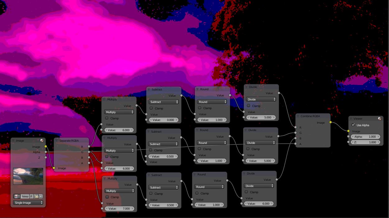
To implement this function in Blender, consider the node setup above. First, feed the image to the Separate RGB node. For the Red channel, we string the math nodes into a function that takes each red color, multiplies (scales) it up by the desired number of divisions (6), offsets it by 0.5, rounds the value to the nearest whole number, and then divides the image pixel color by 5. So, the transformation is {0 to 1} becomes {0 to 6}, subtracting centers the medians to {-0.5 to 5.5} and the rounding to the nearest whole number produces {0, 1, 2, 3, 4, 5} since the function rounds down, and then dividing by five results in six values {0.0, 0.2, 0.4, 0.6, 0.8, 1.0}.
The result is that the output value can only be one of a certain set of values, stair-stepped, because of the rounding function of the math node node setup. Copying this one channel to operate on Green and Blue gives the node setup below. To get the 6:6:7, we set the three Multiply Nodes to {6, 6, 7} and the divide nodes to {5, 5, 6}.
If you make this into a node group, you can easily re-use this setup from project to project. When you do, consider using a math node to drive the different values that you would have to otherwise set manually, just to error-proof your work.
Summary
Normally, an output render consists of 32- or 24-bit color depth, and each pixel can be one of the millions of possible colors. This node setup example takes each of the Red, Green and Blue channels and normalizes them to one of a few values. When all three channels are combined back together, each color can only be one of 256 possible values.
While this example uses the Separate/Combine RGB to create distinct colors, other Separate/Combine nodes can be used as well. If using the YUV values, remember that U and V vary between (-0.5 to +0.5), so you will have to first add on a half to bring the range between 0 and 1, and then after dividing, subtract a half to bring in back into standard range.
The JPG or PNG image format will store each of the colors according to their image standard
for color depth (e.g. JPG is 24-bit), but the image will be very very small since reducing
color depth and quantizing colors are essentially what the JPEG compression algorithm
accomplishes.
You do not have to reduce the color depth of each channel evenly. For example, if blue was the dominant color in an image, to preserve image quality, you could reduce Red to 2 values, Green to 4, and let the blue take on \(256/(2 × 4)\) or 32 values. If using the HSV, you could reduce the Saturation and Value to 2 values (0 or 1.0) by Multiply by 2 and Divide by 2, and restrict the Hue to 64 possible values.
You can use this node setup to quantize any channel; alpha, speed (vector), z-values, and so forth.